Autonomous Lane-Keeping Car Using Raspberry Pi and OpenCV

In this instructables, an autonomous lane keeping robot will be implemented and will pass through the following steps:

• Gathering Parts
• Installing software prerequisites
• Hardware assembly
• First Test
• Detecting lane lines and displaying the guiding line using openCV
• Implementing a PD controller
• Results

The images above show all the components used in this project:

• RC car: I got mine from a local shop in my country. It is equipped with 3 motors (2 for throttling and 1 for steering). The main disadvantage of this car is that the steering is limited between "no steering" and "full steering". In other words, it can not steer at a specific angle, unlike servo-steering RC cars. You can find similar car kit designed specially for raspberry pi from here.
• Raspberry pi 3 model b+: this is the brain of the car which will handle a lot of processing stages. It is based on a quad core 64-bit processor clocked at 1.4 GHz. I got mine from here.
• Raspberry pi 5 mp camera module: It supports 1080p @ 30 fps, 720p @ 60 fps, and 640x480p 60/90 recording. It also supports serial interface which can be plugged directly into the raspberry pi. It is not the best option for image processing applications but it is sufficient for this project as well as it is very cheap. I got mine from here.
• Motor Driver: Is used to control the directions and speeds of the DC motors. It supports the control of 2 dc motors in 1 board and can withstand 1.5 A.
• Power Bank(Optional): I used a power bank (rated at 5V, 3A) to power up the raspberry pi separately. A step down converter (buck converter: 3A output current) should be used in order to power up the raspberry pi from 1 source.
• 3s(12 V) LiPo battery: Lithium Polymer batteries are known for their excellent performance in robotics field. It is used to power the motor driver. I bought mine from here.
• Male to male and female to female jumper wires.
• Double sided tape: Used to mount the components on the RC car.
• Blue tape: This is a very important component of this project, it is used to make the two lane lines in which the car will drive between. You can choose any color you want but I recommend choosing colors different than those in the environment around.
• Zip ties and wood bars.
• Screw driver.

This step is a bit annoying and will take some time.

OpenCV (Open source Computer Vision) is an open source computer vision and machine learning software library. The library has over than 2500 optimized algorithms. Follow THIS very straightforward guide to install the openCV on your raspberry pi as well as installing the raspberry pi OS (if you still didn't). Please note that the process of building the openCV may take around 1.5 hours in a well-cooled room (since the processor's temperature will get very high!) so have some tea and wait patiently :D.

For the remote display, also follow THIS guide to setup remote access to your raspberry pi from your Windows/Mac device.

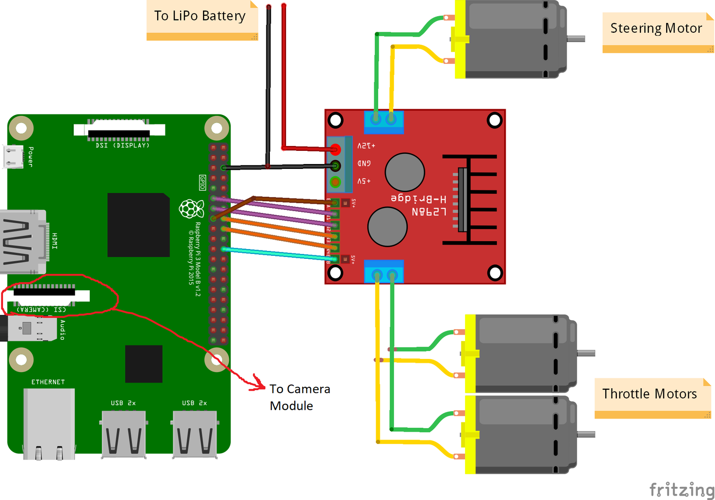
The images above show the connections between raspberry pi, camera module and motor driver. Please note that the motors I used absorb 0.35 A at 9 V each which make it safe for the motor driver to run 3 motors at the same time. And since I want to control the 2 throttling motors' speed (1 rear and 1 front) exactly the same way,I connected them to the same port. I mounted the motor driver on the right side of the car using double tape. As for the camera module, I did insert a zip tie between the screw holes as the image above shows. Then, I fit the camera to a wood bar so that I can adjust the position of the camera as I want. Try to install the camera in the middle of the car as much as possible. I recommend placing the camera at least 20 cm above the ground so the field of view in front of the car will get better. The Fritzing schematic is attached below.

Camera Testing:

Once the camera is installed, and openCV library is built, it's time to test our first image! We will take a photo from pi cam and save it as "original.jpg". It can be done in 2 ways:

1. Using Terminal Commands:

Open a new terminal window and type the following command:

raspistill -o original.jpg 

This will take a still image and save it in "/pi/original.jpg" directory.

2. Using any python IDE (I use IDLE):

Open a new sketch and write the following code:

import cv2

video = cv2.VideoCapture(0)

while True:
  ret,frame = video.read()
  frame = cv2.flip(frame,-1) # used to flip the image vertically
  cv2.imshow('original',frame)
  cv2.imwrite('original.jpg',frame)

  key = cv2.waitKey(1)
  if key == 27:
     break

video.release()
cv2.destroyAllWindows()

Let's see what happened in this code. The first line is importing our openCV library to use all its functions. the VideoCapture(0) function starts streaming a live video from the source determined by this function, in this case it is 0 which means raspi camera. if you have multiple cameras, different numbers should be placed. video.read() will read each frame comes from the camera and save it in a variable called "frame". flip() function will flip the image with respect to y-axis (vertically) since I'm mounting my camera inversely. imshow() will display our frames headed by the word "original" and imwrite() will save our photo as original.jpg. waitKey(1) will wait for 1 ms for any keyboard button to be pressed and returns its ASCII code. if escape (esc) button is pressed, a decimal value of 27 is returned and will break the loop accordingly. video.release() will stop recording and destroyAllWindows() will close every image opened by imshow() function.

I recommend testing your photo with the second method to get familiar with openCV functions.The image is saved in "/pi/original.jpg" directory. The original photo my camera took is shown above.

Testing Motors:

This step is essential to determine the direction of rotation of each motor. First, let's have a brief introduction on the working principle of a motor driver. The image above shows the motor driver pin-out. Enable A, Input 1 and Input 2 are associated with motor A control. Enable B, Input 3 and Input 4 are associated with motor B control. Direction control is established by "Input" part and speed control is established by "Enable" part. To control the direction of motor A for example, set Input 1 to HIGH (3.3 V in this case since we are using a raspberry pi) and set Input 2 to LOW, the motor will spin in a specific direction and by setting the opposite values to Input 1 and Input 2, the motor will spin in the opposite direction. If Input 1 = Input 2 = (HIGH or LOW), the motor won't turn. Enable pins take a Pulse Width Modulation (PWM) input signal from the raspberry (0 to 3.3 V) and run the motors accordingly. For example, a 100% PWM signal means we are working on the maximum speed and 0% PWM signal means the motor is not rotating. The following code is used to determine motors' directions and test their speeds.

import time
import RPi.GPIO as GPIO

GPIO.setwarnings(False)


# Steering Motor Pins
steering_enable = 22 # Physical Pin 15
in1 = 17 # Physical Pin 11
in2 = 27 # Physical Pin 13

#Throttle Motors Pins
throttle_enable = 25 # Physical Pin 22
in3 = 23 # Physical Pin 16
in4 = 24 # Physical Pin 18

GPIO.setmode(GPIO.BCM) # Use GPIO numbering instead of physical numbering
GPIO.setup(in1, GPIO.out)
GPIO.setup(in2, GPIO.out)
GPIO.setup(in3, GPIO.out)
GPIO.setup(in4, GPIO.out)
GPIO.setup(throttle_enable, GPIO.out)
GPIO.setup(steering_enable, GPIO.out)

# Steering Motor Control
GPIO.output(in1, GPIO.HIGH)
GPIO.output(in2, GPIO.LOW)
steering = GPIO.PWM(steering_enable, 1000) # set the switching frequency to 1000 Hz
steering.stop()

# Throttle Motors Control
GPIO.output(in3, GPIO.HIGH)
GPIO.output(in4, GPIO.LOW)
throttle = GPIO.PWM(throttle_enable, 1000) # set the switching frequency to 1000 Hz
throttle.stop()

time.sleep(1)

throttle.start(25) # starts the motor at 25% PWM signal-> (0.25 * battery Voltage) - driver's loss
steering.start(100) # starts the motor at 100% PWM signal-> (1 * Battery Voltage) - driver's loss

time.sleep(3)

throttle.stop()
steering.stop()

This code will run the throttling motors and steering motor for 3 seconds and then will stop them. The (driver's loss) can be determined using a voltmeter. For example, we know that a 100% PWM signal should give the full battery's voltage at the motor's terminal. But, by setting PWM to 100%, I found that the driver is causing a 3 V drop and the motor is getting 9 V instead of 12 V (exactly what I need!). The loss is not linear i.e. the loss at 100% is very different from the loss at 25%. After running the above code, my results were as follow:

Throttling Results: if in3 = HIGH and in4 = LOW, the throttling motors will have a Clock-Wise (CW) rotation i.e. the car will move forward. Otherwise, the car will move backwards.

Steering Results: if in1 = HIGH and in2 = LOW, the steering motor will turn at its maximum left i.e. the car will steer to left. Otherwise, the car will steer right. After some experiments, I found that the steering motor won't turn if the PWM signal was not 100% (i.e. the motor will steer either fully to the right or fully to the left).

In this step, the algorithm that will control the car's movement will be explained. The first image shows the whole process. The input of the system is images, the output is theta (steering angle in degrees). Note that, the processing is done on 1 image and will be repeated on all frames.

Camera:

The camera will start recording a video with (320 x 240) resolution. I recommend lowering the resolution so you can get better frame rate (fps) since fps drop will occur after applying processing techniques to each frame. The code below will be the main loop of the program and will add each step over this code.

import cv2
import numpy as np

video = cv2.VideoCapture(0)
video.set(cv2.CAP_PROP_FRAME_WIDTH,320) # set the width to 320 p
video.set(cv2.CAP_PROP_FRAME_HEIGHT,240) # set the height to 240 p

# The loop
while True:
  ret,frame = video.read()
  frame = cv2.flip(frame, -1)
  cv2.imshow("original",frame)

  key = cv2.waitKey(1)
  if key == 27:
    break

video.release()
cv2.destroyAllWindows()

The code here will show the original image obtained in step 4 and is shown in the images above.

Convert to HSV Color Space:

Now after taking video recording as frames from the camera, the next step is to convert each frame into Hue, Saturation, and Value (HSV) color space. The main advantage of doing so is to be able to differentiate between colors by their level of luminance. And here is a good explanation of HSV color space. Converting to HSV is done via the following function:

def convert_to_HSV(frame):
  hsv = cv2.cvtColor(frame, cv2.COLOR_BGR2HSV)
  cv2.imshow("HSV",hsv)
  return hsv

This function will be called from the main loop and will return the frame in HSV color space. The frame obtained by me in HSV color space is shown above.

Detect Blue Color and Edges:

After converting the image into HSV color space, it's time to detect only the color we are interested about (i.e. blue color since it is the color of the lane lines). To extract blue color from a HSV frame, a range of hue, saturation and value should be specified. refer here to have a better idea on HSV values. After some experiments, the upper and lower limits of blue color are shown in the code below. And to reduce the overall distortion in each frame, edges are detected only using canny edge detector. More about canny edge is found here. A rule of thumb is to select the parameters of Canny() function with a ratio of 1:2 or 1:3.

def detect_edges(frame):
    lower_blue = np.array([90, 120, 0], dtype = "uint8") # lower limit of blue color
    upper_blue = np.array([150, 255, 255], dtype="uint8") # upper limit of blue color
    mask = cv2.inRange(hsv,lower_blue,upper_blue) # this mask will filter out everything but blue

    # detect edges
    edges = cv2.Canny(mask, 50, 100) 
    cv2.imshow("edges",edges)
    return edges

This function will also be called from the main loop which takes as a parameter the HSV color space frame and returns the edged frame. The edged frame I did obtain is found above.

Select Region of Interest (ROI):

Selecting region of interest is crucial to focus only on 1 region of the frame. In this case, I don't want the car to see a lot of items in the environment. I just want the car to focus on the lane lines and ignore anything else. P.S: the coordinate system (x and y axes) starts from the upper left corner. In other words, the point (0,0) starts from the upper left corner. y-axis being the height and x-axis being the width. The code below selects region of interest to focus only on the lower half of the frame.

def region_of_interest(edges):
    height, width = edges.shape # extract the height and width of the edges frame
    mask = np.zeros_like(edges) # make an empty matrix with same dimensions of the edges frame

    # only focus lower half of the screen
    # specify the coordinates of 4 points (lower left, upper left, upper right, lower right)
    polygon = np.array([[
        (0, height), 
        (0,  height/2),
        (width , height/2),
        (width , height),
    ]], np.int32)

    cv2.fillPoly(mask, polygon, 255) # fill the polygon with blue color 
    cropped_edges = cv2.bitwise_and(edges, mask) 
    cv2.imshow("roi",cropped_edges)
    return cropped_edges

This function will take the edged frame as parameter and draws a polygon with 4 preset points. It will only focus on what's inside the polygon and ignore everything outside it. My region of interest frame is shown above.

Detect Line Segments:

Hough transform is used to detect line segments from an edged frame. Hough transform is a technique to detect any shape in mathematical form. It can detect nearly any object even if its distorted according to some number of votes. a great reference for Hough transform is shown here. For this application, cv2.HoughLinesP() function is used to detect lines in each frame. The important parameters this function take are:

cv2.HoughLinesP(frame, rho, theta, min_threshold, minLineLength, maxLineGap)

• Frame: is the frame we want to detect lines in.
• rho: It is the the distance precision in pixels (usually it is = 1)
• theta: angular precision in radians ( always = np.pi/180 ~ 1 degree)
• min_threshold: minimum vote it should get for it to be considered as a line
• minLineLength: minimum length of line in pixels. Any line shorter than this number is not considered a line.
• maxLineGap: maximum gap in pixels between 2 lines to be treated as 1 line. (It is not used in my case since the lane lines I am using don't have any gap).

This function returns the endpoints of a line. The following function is called from my main loop to detect lines using Hough transform:

def detect_line_segments(cropped_edges):
    rho = 1  
    theta = np.pi / 180  
    min_threshold = 10 
    line_segments = cv2.HoughLinesP(cropped_edges, rho, theta, min_threshold, 
                                    np.array([]), minLineLength=5, maxLineGap=0)
    return line_segments

Average slope and Intercept (m, b):

recall that the equation of line is given by y = mx + b. Where m is the slope of the line and b is the y-intercept. In this part, the average of slopes and intercepts of line segments detected using Hough transform will be calculated. Before doing so, let's take a look on the original frame photo shown above. The left lane appears to be going upwards so it has a negative slope (remember the coordinate system start point?). In other words, the left lane line has x1 < x2 and y2 < y1 and the slope = (y2 - y1) / (x2 - x1) which will give a negative slope. Therefore, all lines with negative slopes are considered left lane points. The right lane is the complete opposite, we can see that the right lane is going downwards and will have positive slope. Right lane has x2 > x1 and y2 > y1 which will give a positive slope. So, all lines with positive slope are considered right lane points. In case of vertical lines (x1 = x2), the slope will be infinity. In this case, we will skip all vertical lines to prevent getting an error. To add more accuracy to this detection, each frame is divided into two regions (right and left) through 2 boundary lines. All width points (x-axis points) greater than right boundary line, are associated with right lane calculation. And if all width points are less than the left boundary line, they are associated with left lane calculation. The following function takes the frame under processing and lane segments detected using Hough transform and returns the average slope and intercept of two lane lines.

def average_slope_intercept(frame, line_segments):
    lane_lines = []

    if line_segments is None:
        print("no line segment detected")
        return lane_lines

    height, width,_ = frame.shape
    left_fit = []
    right_fit = []
    boundary = 1/3

    left_region_boundary = width * (1 - boundary) 
    right_region_boundary = width * boundary 

    for line_segment in line_segments:
        for x1, y1, x2, y2 in line_segment:
            if x1 == x2:
                print("skipping vertical lines (slope = infinity)")
                continue

            fit = np.polyfit((x1, x2), (y1, y2), 1)
            slope = (y2 - y1) / (x2 - x1)
            intercept = y1 - (slope * x1)

            if slope < 0:
                if x1 < left_region_boundary and x2 < left_region_boundary:
                    left_fit.append((slope, intercept))
            else:
                if x1 > right_region_boundary and x2 > right_region_boundary:
                    right_fit.append((slope, intercept))

    left_fit_average = np.average(left_fit, axis=0)
    if len(left_fit) > 0:
        lane_lines.append(make_points(frame, left_fit_average))

    right_fit_average = np.average(right_fit, axis=0)
    if len(right_fit) > 0:
        lane_lines.append(make_points(frame, right_fit_average))

    # lane_lines is a 2-D array consisting the coordinates of the right and left lane lines
    # for example: lane_lines = [[x1,y1,x2,y2],[x1,y1,x2,y2]]
    # where the left array is for left lane and the right array is for right lane 
    # all coordinate points are in pixels
    return lane_lines

make_points() is a helper function for average_slope_intercept() function which will return the bounded coordinates of the lane lines (from the bottom to the middle of the frame).

def make_points(frame, line):
    height, width, _ = frame.shape
    slope, intercept = line
    y1 = height  # bottom of the frame
    y2 = int(y1 / 2)  # make points from middle of the frame down

    if slope == 0: 
        slope = 0.1    

    x1 = int((y1 - intercept) / slope)
    x2 = int((y2 - intercept) / slope)

    return [[x1, y1, x2, y2]]

To prevent dividing by 0, a condition is presented. If slope = 0 which means y1 = y2 (horizontal line) , give the slope a value near 0. This will not affect the performance of the algorithm as well as it will prevent impossible case (dividing by 0).

To display the lane lines on the frames, the following function is used:

def display_lines(frame, lines, line_color=(0, 255, 0), line_width=6): # line color (B,G,R)
    line_image = np.zeros_like(frame)

    if lines is not None:
        for line in lines:
            for x1, y1, x2, y2 in line:
                cv2.line(line_image, (x1, y1), (x2, y2), line_color, line_width)

    line_image = cv2.addWeighted(frame, 0.8, line_image, 1, 1)  
    return line_image

cv2.addWeighted() function takes the following parameters and it is used to combine two images but with giving each one a weight.

cv2.addWeighted(image1, alpha, image2, beta, gamma) 

And calculates the output image using the following equation:

output = alpha * image1 + beta * image2 + gamma

More information about cv2.addWeighted() function are derived here.

Calculate and Display Heading Line:

This is the final step before we apply speeds to our motors. The heading line is responsible to give the steering motor the direction in which it should rotate and give the throttling motors the speed at which they will operate. Calculating heading line is pure trigonometry, tan and atan (tan^-1) trigonometric functions are used. Some extreme cases are when the camera detects only one lane line or when it doesn't detect any line. All these cases are shown in the following function:

def get_steering_angle(frame, lane_lines):
     height, width, _ = frame.shape

     if len(lane_lines) == 2: # if two lane lines are detected
        _, _, left_x2, _ = lane_lines[0][0] # extract left x2 from lane_lines array
        _, _, right_x2, _ = lane_lines[1][0] # extract right x2 from lane_lines array
        mid = int(width / 2)
        x_offset = (left_x2 + right_x2) / 2 - mid
        y_offset = int(height / 2)  

    elif len(lane_lines) == 1: # if only one line is detected
        x1, _, x2, _ = lane_lines[0][0]
        x_offset = x2 - x1
        y_offset = int(height / 2)

    elif len(lane_lines) == 0: # if no line is detected
        x_offset = 0
        y_offset = int(height / 2)

    angle_to_mid_radian = math.atan(x_offset / y_offset)
    angle_to_mid_deg = int(angle_to_mid_radian * 180.0 / math.pi)  
    steering_angle = angle_to_mid_deg + 90 

    return steering_angle

x_offset in the first case is how much the average ((right x2 + left x2) / 2) differs from the middle of the screen. y_offset is always taken to be height / 2. The last image above shows an example of heading line. angle_to_mid_radians is the same as "theta" shown in the last image above. If steering_angle = 90, it means that the car has a heading line perpendicular to "height / 2" line and the car will move forward without steering. If steering_angle > 90, the car should steer to right otherwise it should steer left. To display the heading line, the following function is used:

def display_heading_line(frame, steering_angle, line_color=(0, 0, 255), line_width=5 )

    heading_image = np.zeros_like(frame)
    height, width, _ = frame.shape

    steering_angle_radian = steering_angle / 180.0 * math.pi
    x1 = int(width / 2)
    y1 = height
    x2 = int(x1 - height / 2 / math.tan(steering_angle_radian))
    y2 = int(height / 2)

    cv2.line(heading_image, (x1, y1), (x2, y2), line_color, line_width)

    heading_image = cv2.addWeighted(frame, 0.8, heading_image, 1, 1)

    return heading_image

The function above takes the frame in which the heading line will be drawn on and steering angle as input. It returns the image of the heading line. The heading line frame taken in my case is shown in the image above.

Combining All Code Together:

The code now is ready to be assembled. The following code shows the main loop of the program calling each function:

import cv2
import numpy as np

video = cv2.VideoCapture(0)
video.set(cv2.CAP_PROP_FRAME_WIDTH,320)
video.set(cv2.CAP_PROP_FRAME_HEIGHT,240)

while True:
    ret,frame = video.read()
    frame = cv2.flip(frame,-1)

    #Calling the functions
    hsv = convert_to_HSV(frame)
    edges = detect_edges(hsv)
    roi = region_of_interest(edges)
    line_segments = detect_line_segments(roi)
    lane_lines = average_slope_intercept(frame,line_segments)
    lane_lines_image = display_lines(frame,lane_lines)
    steering_angle = get_steering_angle(frame, lane_lines)
    heading_image = display_heading_line(lane_lines_image,steering_angle)

    key = cv2.waitKey(1)
    if key == 27:
        break

video.release()
cv2.destroyAllWindows()

Now we have our steering angle ready to be fed to the motors. As mentioned earlier, if steering angle is greater than 90, the car should turn right otherwise it should turn left. I applied a simple code that turns the steering motor right if the angle is above 90 and turns it left if steering angle is less than 90 at a constant throttling speed of (10% PWM) but I got a lot of errors. The main error I got is when the car approaches any turn, the steering motor acts directly but the throttling motors get jammed. I tried to increase the throttling speed to be (20% PWM) at turns but ended with the robot getting out of the lanes. I needed something that increases the throttling speed a lot if the steering angle is very big and increases the speed a bit if the steering angle is not that big then decreases the speed to an initial value as the car approaches 90 degrees (moving straight). The solution was to use a PD controller.

PID controller stands for Proportional, Integral and Derivative controller. This type of linear controllers is widely used in robotics applications. The image above shows the typical PID feedback control loop. The goal of this controller is to reach the "setpoint" with the most efficient way unlike "on - off" controllers which turn on or off the plant according to some conditions. Some keywords should be known:

• Setpoint: is the desired value you want your system to reach.
• Actual value: is the actual value sensed by sensor.
• Error: is the difference between setpoint and actual value (error = Setpoint - Actual value).
• Controlled variable: from its name, the variable you wish to control.
• Kp: Proportional constant.
• Ki: Integral constant.
• Kd: Derivative constant.

In short, the PID control system loop works as follows:

• The user defines the setpoint needed for the system to reach.
• The error is calculated (error = setpoint - actual).
• P controller generates an action proportional to error's value. (error increases, P action also increases)
• I controller will integrate the error over time which eliminates the system's steady state error but increases its overshoot.
• D controller is simply the time derivative for the error. In other words, it is the slope of the error. It does an action proportional to the derivative of the error. This controller increases the stability of the system.
• The output of the controller will be the sum of the three controllers. The controller's output will become 0 if the error becomes 0.

A great explanation of PID controller can be found here.

Going back to the lane keeping car, my controlled variable was throttling speed (since steering has only two states either right or left). A PD controller is used for this purpose since D action increases the throttling speed a lot if the error change is very big (i.e. large deviation) and slows down the car if this error change approaches 0. I did the following steps to implement a PD controller:

• Set the setpoint to 90 degrees (I always want the car to move straight)
• Calculated the deviation angle from middle
• The deviation gives two information: How big the error is (magnitude of deviation) and what direction the steering motor has to take (sign of deviation). If deviation is positive, the car should steer right otherwise it should steer left.
• Since deviation is either negative or positive, an "error" variable is defined and always equal to the absolute value of the deviation.
• The error is multiplied by a constant Kp.
• The error undergoes time differentiation and is multiplied by a constant Kd.
• Motors' speed is updated and the loop starts again.

The following code is used in the main loop to control the throttling motors' speed:

speed = 10 # operating speed in % PWM

#Variables to be updated each loop
lastTime = 0 
lastError = 0

# PD constants
Kp = 0.4
Kd = Kp * 0.65

While True:
    now = time.time() # current time variable
    dt = now - lastTime
    deviation = steering_angle - 90 # equivalent to angle_to_mid_deg variable
    error = abs(deviation) 

    if deviation < 5 and deviation > -5: # do not steer if there is a 10-degree error range
        deviation = 0
        error = 0
        GPIO.output(in1,GPIO.LOW)
        GPIO.output(in2,GPIO.LOW)
        steering.stop()

    elif deviation > 5: # steer right if the deviation is positive
        GPIO.output(in1,GPIO.LOW)
        GPIO.output(in2,GPIO.HIGH)
        steering.start(100)

    elif deviation < -5: # steer left if deviation is negative
        GPIO.output(in1,GPIO.HIGH)
        GPIO.output(in2,GPIO.LOW)
        steering.start(100)

    derivative = kd * (error - lastError) / dt 
    proportional = kp * error
    PD = int(speed + derivative + proportional)

    spd = abs(PD)
    if spd > 25:
       spd = 25

    throttle.start(spd)

    lastError = error
    lastTime = time.time()

If error is very big (the deviation from middle is high), the proportional and derivative actions are high resulting in high throttling speed. When error approaches 0 (deviation from middle is low), the derivative action acts reversely (slope is negative) and the throttling speed gets low to maintain stability of the system. The full code is attached below.

The videos above show the results I obtained. It does need more tuning and further adjustments. I was connecting the raspberry pi to my LCD display screen because the video streaming over my network had high latency and was very frustrating to work with, that is why there are wires connected to raspberry pi in the video. I used foam boards to draw the track on.

I am waiting to hear your recommendations to make this project better! As I hope that this instructables was good enough to give you some new information.